
How Transformers Architecture Powers Modern LLMs

Why context engines matter more than models in 2026 (Sponsored)

One of the clearest AI predictions for 2026: models won’t be the bottleneck—context will. As AI agents pull from vector stores, session state, long-term memory, SQL, and more, finding the right data becomes the hard part. Miss critical context and responses fall apart. Send too much and latency and costs spike.
Context engines emerge as the fix. A single layer to store, index, and serve structured and unstructured data, across short- and long-term memory. The result: faster responses, lower costs, and AI apps that actually work in production.
When we interact with modern large language models like GPT, Claude, or Gemini, we are witnessing a process fundamentally different from how humans form sentences. While we naturally construct thoughts and convert them into words, LLMs operate through a cyclical conversion process.
Understanding this process reveals both the capabilities and limitations of these powerful systems.
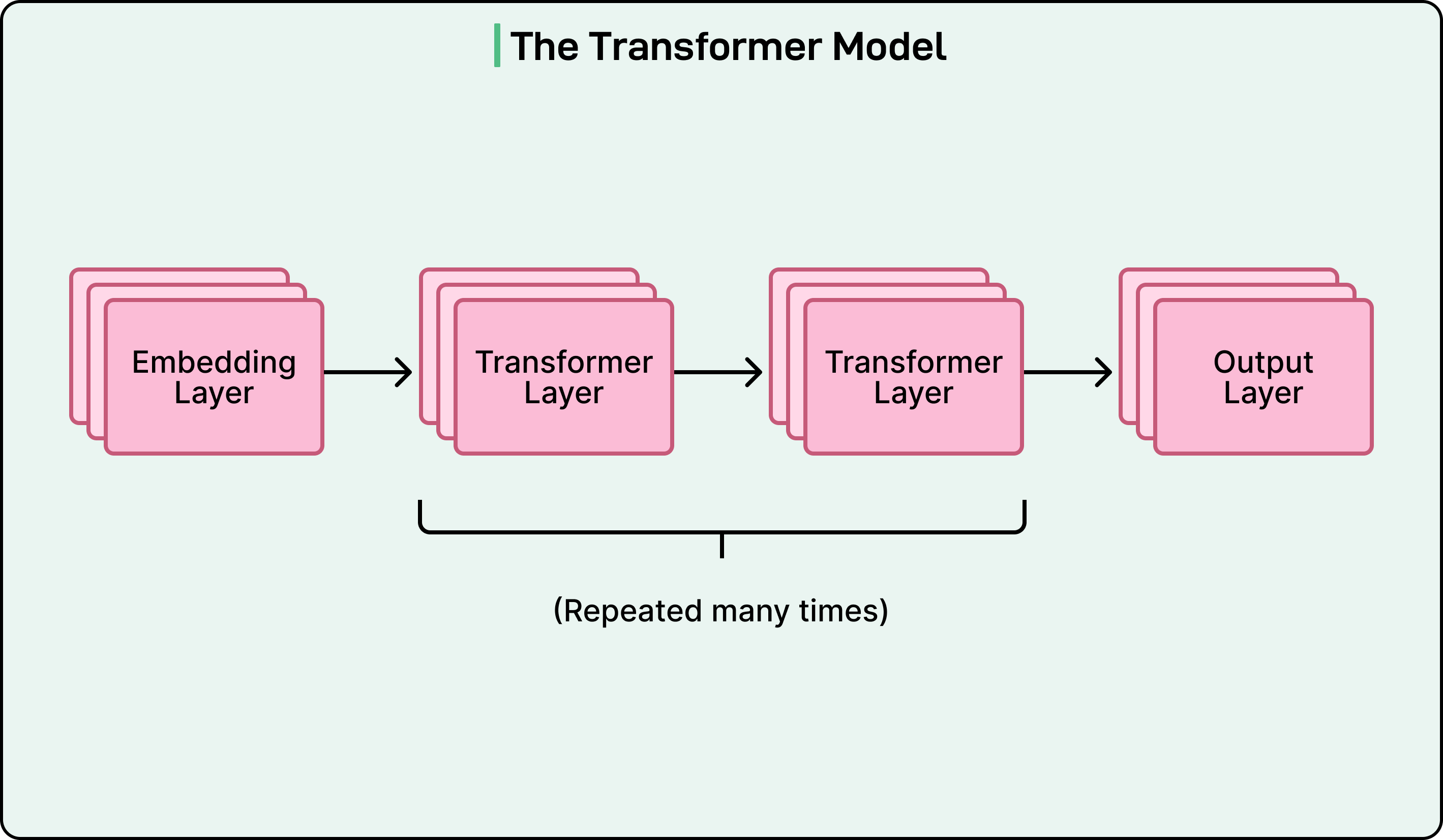
At the heart of most modern LLMs lies an architecture called a transformer. Introduced in 2017, transformers are sequence prediction algorithms built from neural network layers. The architecture has three essential components:
An embedding layer that converts tokens into numerical representations.
Multiple transformer layers where computation happens.
Output layer that converts results back into text.
See the diagram below:
Transformers process all words simultaneously rather than one at a time, enabling them to learn from massive text datasets and capture complex word relationships.
In this article, we will look at how the transformer architecture works in a step-by-step manner.
Step 1: From Text to Tokens
Before any computation can happen, the model must convert text into a form it can work with. This begins with tokenization, where text gets broken down into fundamental units called tokens. These are not always complete words. They can be subwords, word fragments, or even individual characters.
Consider this example input: “I love transformers!” The tokenizer might break this into: [”I”, “ love”, “ transform”, “ers”, “!”]. Notice that “transformers” became two separate tokens. Each unique token in the vocabulary gets assigned a unique integer ID:
“I” might be token 150
“love” might be token 8942
“transform” might be token 3301
“ers” might be token 1847
“!” might be token 254
These IDs are arbitrary identifiers with no inherent relationships. Tokens 150 and 151 are not similar just because their numbers are close. The overall vocabulary typically contains 50,000 to 100,000 unique tokens that the model learned during training.
Step 2: Converting Tokens to Embeddings
Neural networks cannot work directly with token IDs because they are just fixed identifiers. Each token ID gets mapped to a vector, a list of continuous numbers usually containing hundreds or thousands of dimensions. These are called embeddings.
Here is a simplified example with five dimensions (real models may use 768 to 4096):
Token “dog” becomes [0.23, -0.67, 0.45, 0.89, -0.12]
Token “wolf” becomes [0.25, -0.65, 0.47, 0.91, -0.10]
Token “car” becomes [-0.82, 0.34, -0.56, 0.12, 0.78]
Notice how “dog” and “wolf” have similar numbers, while “car” is completely different. This creates a semantic space where related concepts cluster together.
Why the need for multiple dimensions? This is because with just one number per word, we might encounter contradictions. For example:
“stock” equals 5.2 (financial term)
“capital” equals 5.3 (similar financial term)
“rare” equals -5.2 (antonym: uncommon)
“debt” equals -5.3 (antonym of capital)
Now, “rare” and “debt” both have similar negative values, implying they are related, which makes no sense. Hundreds of dimensions allow the model to represent complex relationships without such contradictions.
In this space, we can perform mathematical operations. The embedding for “king” minus “man” plus “woman” approximately equals “queen.” These relationships emerge during training from patterns in text data.
Step 3: Adding Positional Information
Transformers do not inherently understand word order. Without additional information, “The dog chased the cat” and “The cat chased the dog” would look identical because both contain the same tokens.
The solution is positional embeddings. Every position gets mapped to a position vector, just like tokens get mapped to meaning vectors.
For the token “dog” appearing at position 2, it might look like the following:
Word embedding: [0.23, -0.67, 0.45, 0.89, -0.12]
Position 2 embedding: [0.05, 0.12, -0.08, 0.03, 0.02]
Combined (element-wise sum): [0.28, -0.55, 0.37, 0.92, -0.10]
This combined embedding captures both the meaning of the word and its context of use. This is also what flows into the transformer layers.
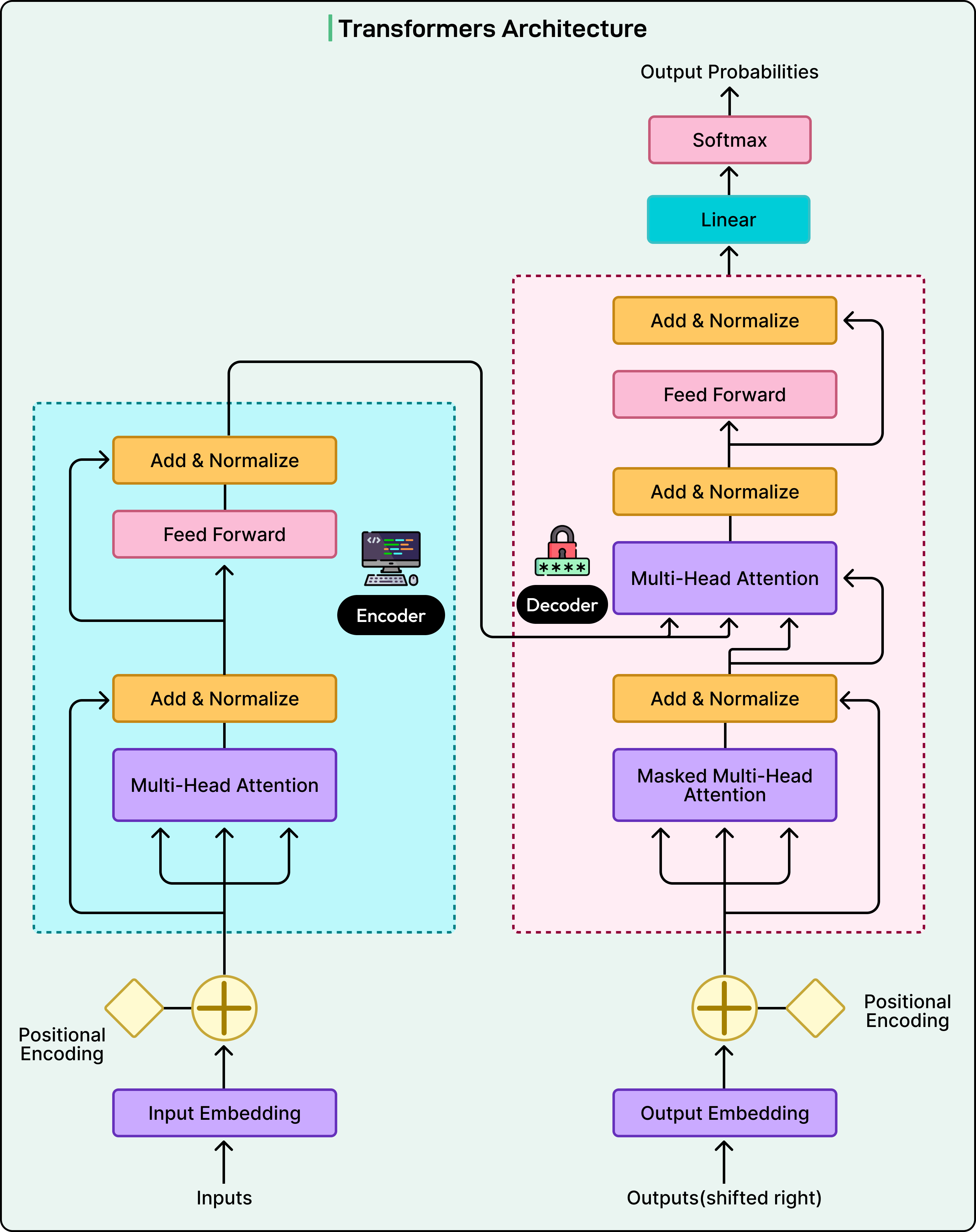
Step 4: The Attention Mechanism in Transformer Layers
The transformer layers implement the attention mechanism, which is the key innovation that makes these models so powerful. Each transformer layer operates using three components for every token: queries, keys, and values. We can think of this as a fuzzy dictionary lookup where the model compares what it is looking for (the query) against all possible answers (the keys) and returns weighted combinations of the corresponding values.
Let us walk through a concrete example. Consider the sentence: “The cat sat on the mat because it was comfortable.”
When the model processes the word “it,” it needs to determine what “it” refers to. Here is what happens:
First, the embedding for “it” generates a query vector asking essentially, “What noun am I referring to?”
Next, this query is compared against the keys from all previous tokens. Each comparison produces a similarity score. For example:
“The” (article) generates score: 0.05
“cat” (noun) generates score: 8.3
“sat” (verb) generates score: 0.2
“on” (preposition) generates score: 0.03
“the” (article) generates score: 0.04
“mat” (noun) generates score: 4.1
“because” (conjunction) generates score: 0.1
The raw scores are then converted into attention weights that sum to 1.0. For example:
“cat” receives attention weight: 0.75 (75 percent)
“mat” receives attention weight: 0.20 (20 percent)
All other tokens: 0.05 total (5 percent combined)
Finally, the model takes the value vectors from each token and combines them using these weights. For example:
Output = (0.75 × Value_cat) + (0.20 × Value_mat) + (0.03 × Value_the) + ...The value from “cat” contributes 75 percent to the output, “mat” contributes 20 percent, and everything else is nearly ignored. This weighted combination becomes the new representation for “it” that captures the contextual understanding that “it” most likely refers to “cat.”
This attention process happens in every transformer layer, but each layer learns to detect different patterns.
Early layers learn basic patterns like grammar and common word pairs. When processing “cat,” these layers might heavily attend to “The” because they learn that articles and their nouns are related.
Middle layers learn sentence structure and relationships between phrases. They might figure out that “cat” is the subject of “sat” and that “on the mat” forms a prepositional phrase indicating location.
Deep layers extract abstract meaning. They might understand that this sentence describes a physical situation and implies the cat is comfortable or resting.
Each layer refines the representation progressively. The output of one layer becomes the input for the next, with each layer adding more contextual understanding.
Importantly, only the final transformer layer needs to predict an actual token. All intermediate layers perform the same attention operations but simply transform the representations to be more useful for downstream layers. A middle layer does not output token predictions. Instead, it outputs refined vector representations that flow to the next layer.
This stacking of many layers, each specializing in different aspects of language understanding, is what enables LLMs to capture complex patterns and generate coherent text.
Step 5: Converting Back to Text
After flowing through all layers, the final vector must be converted to text. The unembedding layer compares this vector against every token embedding and produces scores.
For example, to complete “I love to eat,” the unembedding might produce:
“pizza”: 65.2
“tacos”: 64.8
“sushi”: 64.1
“food”: 58.3
“barbeque”: 57.9
“car”: -12.4
“42”: -45.8
These arbitrary scores get converted to probabilities using softmax:
“pizza”: 28.3 percent
“tacos”: 24.1 percent
“sushi”: 18.9 percent
“food”: 7.2 percent
“barbeque”: 6.1 percent
“car”: 0.0001 percent
“42”: 0.0000001 percent
Tokens with similar scores (65.2 versus 64.8) receive similar probabilities (28.3 versus 24.1 percent), while low-scoring tokens get near-zero probabilities.
The model does not select the highest probability token. Instead, it randomly samples from this distribution. Think of a roulette wheel where each token gets a slice proportional to its probability. Pizza gets 28.3 percent, tacos get 24.1 percent, and 42 gets a microscopic slice.
The reason for this randomness is that always picking a specific value like “pizza” would create repetitive, unnatural output. Random sampling weighted by probability allows selection of “tacos,” “sushi,” or “barbeque,” producing varied, natural responses. Occasionally, a lower-probability token gets picked, leading to creative outputs.
The Iterative Generation Loop
The generation process repeats for every token. Let us walk through an example where the initial prompt is “The capital of France.” Here’s how different cycles go through the transformer:
Cycle 1:
Input: [”The”, “capital”, “of”, “France”]
Process through all layers
Sample: “is” (80 percent)
Output so far: “The capital of France is”
Cycle 2:
Input: [”The”, “capital”, “of”, “France”, “is”] (includes new token)
Process through all layers (5 tokens now)
Sample: “Paris” (92 percent)
Output so far: “The capital of France is Paris”
Cycle 3:
Input: [”The”, “capital”, “of”, “France”, “is”, “Paris”] (6 tokens)
Process through all layers
Sample: “.” (65 percent)
Output so far: “The capital of France is Paris.”
Cycle 4:
Input: [”The”, “capital”, “of”, “France”, “is”, “Paris”, “.”] (7 tokens)
Process through all layers
Sample: [EoS] token (88 percent)
Stop the loop
Final output: “The capital of France is Paris.”
The [EoS] or end-of-sequence token signals completion. Each cycle processes all previous tokens. This is why generation can slow as responses lengthen.
This is called autoregressive generation because each output depends on all previous outputs. If an unusual token gets selected (perhaps “chalk” with 0.01 percent probability in “I love to eat chalk”), all subsequent tokens will be influenced by this choice.
Training Versus Inference: Two Different Modes
The transformer flow operates in two contexts: training and inference.
During training, the model learns language patterns from billions of text examples. It starts with random weights and gradually adjusts them. Here is how training works:
Training text: “The cat sat on the mat.”
Model receives: “The cat sat on the”
With random initial weights, the model might predict:
“banana”: 25 percent
“car”: 22 percent
“mat”: 3 percent (correct answer has low probability)
“elephant”: 18 percent
The training process calculates the error (mat should have been higher) and uses backpropagation to adjust every weight:
Embeddings for “on” and “the” get adjusted
Attention weights in all 96 layers get adjusted
Unembedding layer gets adjusted
Each adjustment is tiny (0.245 to 0.247), but it accumulates across billions of examples. After seeing “sat on the” followed by “mat” thousands of times in different contexts, the model learns this pattern. Training takes weeks on thousands of GPUs and costs millions of dollars. Once complete, weights are frozen.
During inference, the transformer runs with frozen weights:
User query: “Complete this: The cat sat on the”
The model processes the input with its learned weights and outputs: “mat” (85 percent), “floor” (8 percent), “chair” (3 percent). It samples “mat” and returns it. No weight changes occur.
The model used its learned knowledge but did not learn anything new. The conversations do not update model weights. To teach the model new information, we would need to retrain it with new data, which requires substantial computational resources.
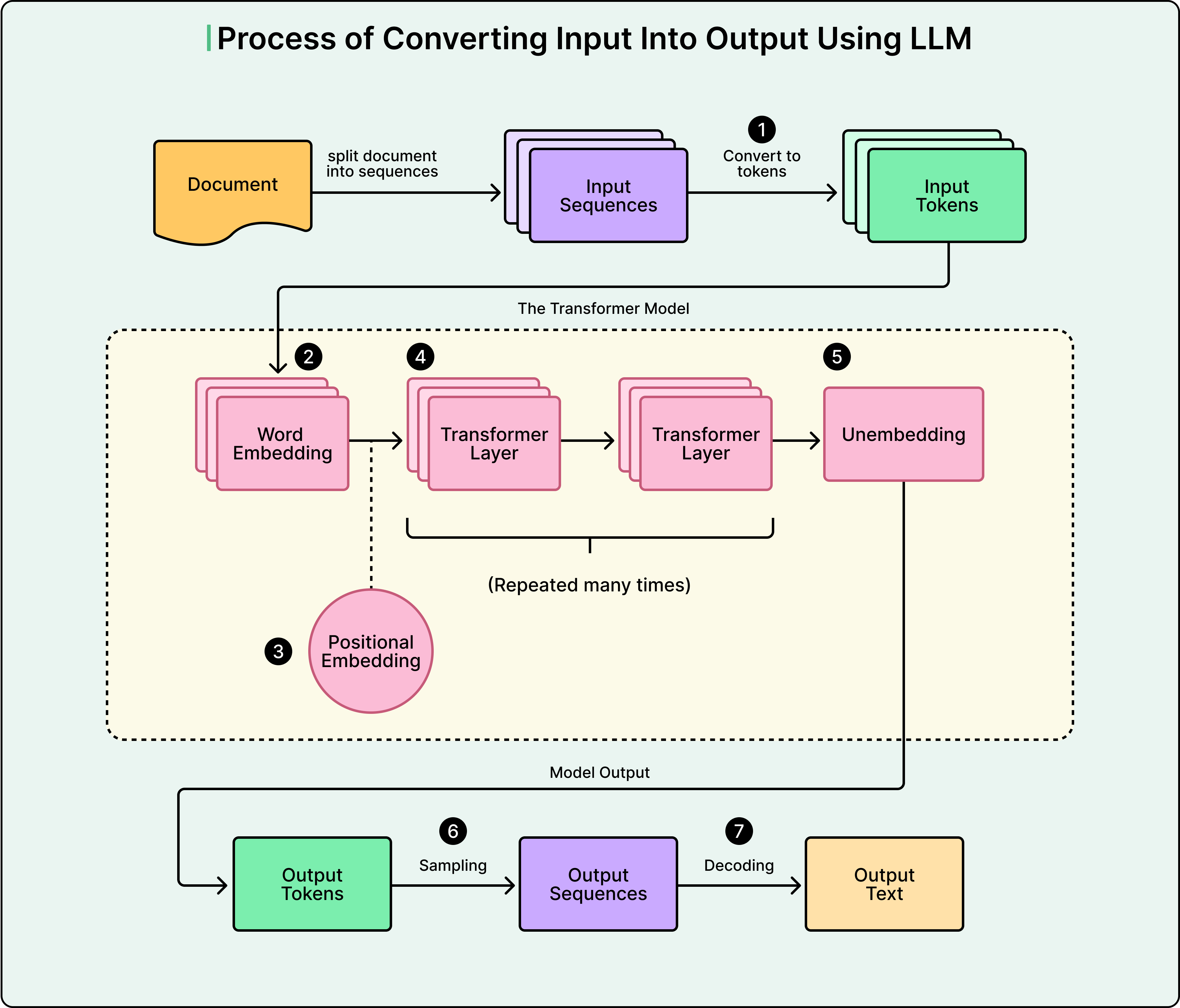
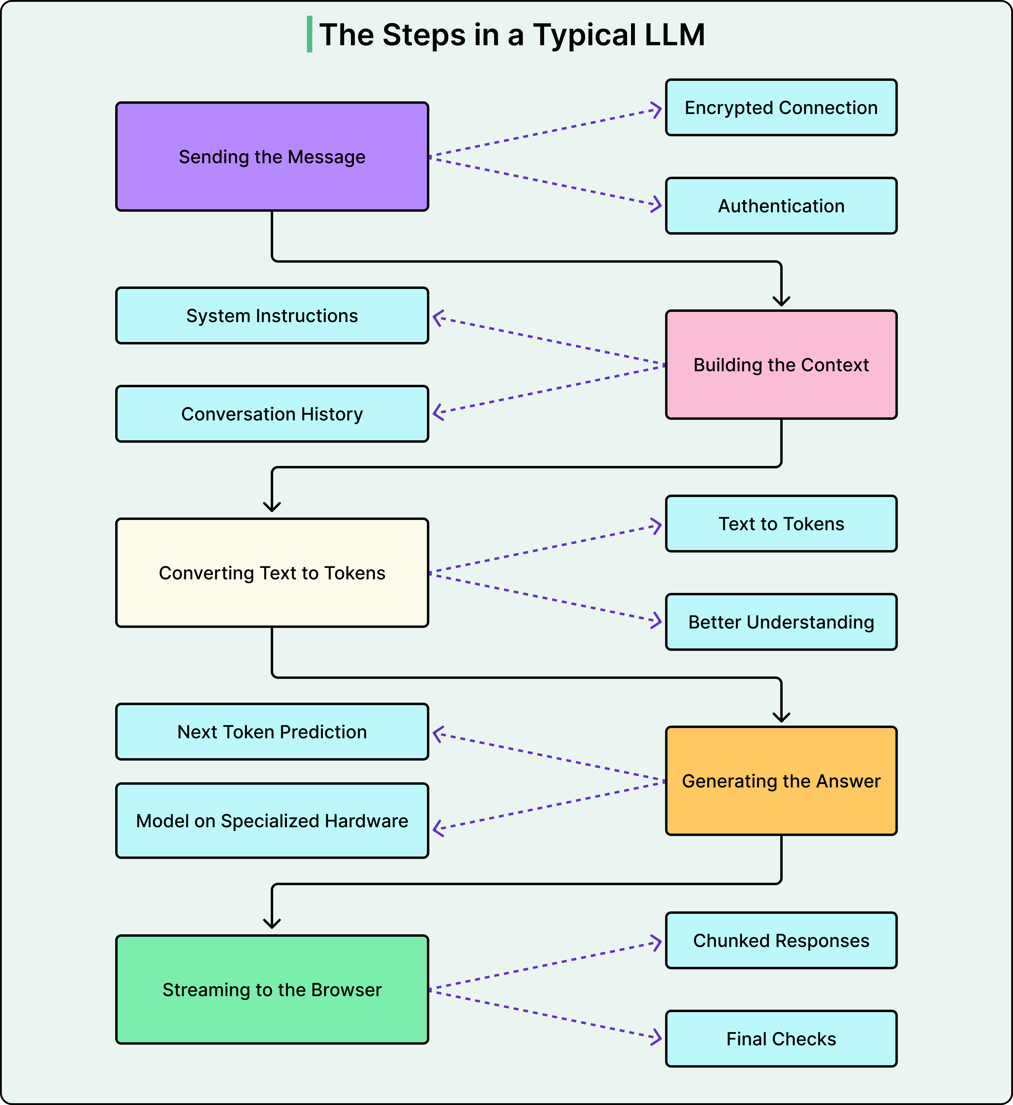
See the diagram below that shows the various steps in an LLM execution flow:
Conclusion
The transformer architecture provides an elegant solution to understanding and generating human language. By converting text to numerical representations, using attention mechanisms to capture relationships between words, and stacking many layers to learn increasingly abstract patterns, transformers enable modern LLMs to produce coherent and useful text.
This process involves seven key steps that repeat for every generated token: tokenization, embedding creation, positional encoding, processing through transformer layers with attention mechanisms, unembedding to scores, sampling from probabilities, and decoding back to text. Each step builds on the previous one, transforming raw text into mathematical representations that the model can manipulate, then back into human-readable output.
Understanding this process reveals both the capabilities and limitations of these systems. In essence, LLMs are sophisticated pattern-matching machines that predict the most likely next token based on patterns learned from massive datasets.
The attention mechanism walkthrough with concrete scores is what makes this click for people. One thing I'd add: understanding that the temperature parameter directly controls that sampling roulette wheel is huge for anyone building on top of LLMs. Lower temperature = tighter distribution = more predictable outputs. I run multiple AI coding agents in production daily, and tuning temperature is the difference between getting reliable code generation vs. creative hallucinations. The autoregressive generation loop also explains why context window management matters so much — every extra token compounds the computation cost.
While this is a solid explanation of transformer architecture and function, your statement regarding how humans "naturally" form throughts and convert them into language is incredibly oversimplified. If you want to compare the similarities and differences between human cognition and LLM function, you actually need to understand how humans cognate and form linguistic representations.
Key Processes in Thought and Speech Generation:
Thought Formation: Complex thoughts emerge from interconnected, dynamic neural patterns that act as a "lightning storm" of activity. These, for the most part, are processed in high-level cognitive, non-verbal areas.
Word Selection & Sequencing: The posterior-superior temporal gyrus (P-STG) serves as a core language hub to select words and arrange them into linguistic structures, transitioning from abstract ideas to linguistic components.
Neural Encoding Cascade: Research indicates a specific, fast-acting sequence where neurons activate:
400 ms before speech: Morphemes (meaning units) activate.
200 ms before speech: Phonemes (consonant/vowel sounds) activate.
70 ms before speech: Syllables (units of pronunciation) activate.
Broca's Area and Motor Cortex: These areas are responsible for planning the speech response and controlling the muscles in the throat, mouth, and lips to produce sound.
Brain-Computer Interfaces (BCI): Researchers have developed technologies that can decode these electrical signals directly from the motor cortex to translate, in near real-time, intended movements of the vocal tract into text or audible speech.
This process involves a hierarchical structure where abstract thoughts are translated into a sequence of linguistic, then acoustic, representations.
Now, we can begin to have a conversation that matters about the differences and similarities between human language generation and LLMs.